2026 Top Types of Machine Vision Inspection Systems

Machine Vision Inspection is becoming a practical quality-control layer across factories, warehouses, and laboratories. Cameras now examine surfaces, labels, dimensions, seals, and assembly positions within milliseconds. In many production lines, this changes inspection from occasional sampling to continuous, documented checking. The technology is not magic, however. Poor lighting, reflective materials, unstable fixtures, and weak image datasets can still produce unreliable decisions.

Industry forecasts show strong commercial momentum. MarketsandMarkets’ Machine Vision Market report projects the global market to grow from approximately USD 12.8 billion in 2024 to USD 17.2 billion by 2029, at a compound annual growth rate of about 6.1%. Grand View Research also expects continued expansion through 2030, driven by automation, robotics, electronics manufacturing, and pharmaceutical quality requirements. These estimates differ because research firms define “machine vision” differently. That difference deserves attention.

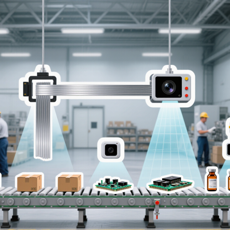
The 2026 Top Types of Machine Vision Inspection Systems guide will compare the main system categories used in modern production. It will examine 2D area-scan systems, line-scan cameras, 3D vision platforms, smart cameras, and vision-guided inspection cells. Each type suits different objects and risks. A line-scan system may reveal a tiny coating gap on moving steel. A 3D camera can detect missing height on a connector. A smart camera may reduce cabinet space, but its processing limits can matter. Real-world performance depends on integration, calibration, maintenance, and operator training—not only camera resolution. Some installations still fail for simple reasons: dust on a lens, changing illumination, or an unclear acceptance threshold. That is where careful engineering matters.

Table of Contents [Hide]

1 2D Area-Scan Systems: 5–25 MP Cameras for Surface and Assembly Inspection

2 Line-Scan Vision Systems: 10–100 kHz Rates for Continuous Web Inspection

3 3D Machine Vision: 3–100 μm Depth Resolution for Height and Volume Measurement

4 Multispectral and Hyperspectral Systems: 4–100+ Bands for Material Sorting

5 AI-Enabled Vision Systems: Precision, Recall, and False-Reject Rates as KPIs

2D Area-Scan Systems: 5–25 MP Cameras for Surface and Assembly Inspection

2D area-scan inspection systems use 5–25 MP cameras to capture complete images of stationary or moving parts. They support surface and assembly inspection across electronics, packaging, machined components, and consumer products. A single frame can reveal scratches, missing components, incorrect labels, gaps, and uneven edges.

At 5 MP, the system may suit larger parts with moderate defect sizes. Higher resolutions expose smaller marks, but they also increase storage, processing, and lighting demands. Resolution alone is not accuracy. The lens, working distance, sensor size, and lighting must work together. Diffused lighting can show shallow dents, while angled lighting may emphasize raised features. The wrong light can hide a defect completely.

A practical setup starts with the smallest defect that must be detected. Engineers should measure it, not estimate it from a sample image. Trigger timing and part positioning also matter, especially on conveyors. Vibration can turn a sharp edge into a blurred line. The system is not perfect. A first design may pass clean samples and fail on reflective parts, dust, or color changes. That failure is useful. It exposes weak assumptions before full deployment. Reliable inspection depends on controlled tests, recorded images, and regular review of false rejects and missed defects.

Line-Scan Vision Systems: 10–100 kHz Rates for Continuous Web Inspection

Line-scan vision systems capture one pixel row at a time, making them suitable for continuous webs, films, metals, paper, and textiles. At 10–100 kHz, they can inspect rapidly moving material while maintaining consistent image spacing. The real requirement is synchronization. An encoder must match line timing with web speed, or defects may stretch, compress, or disappear.

Industry forecasts support this demand. MarketsandMarkets projects the machine vision market to grow from about USD 12.2 billion in 2023 to USD 17.2 billion by 2028. Grand View Research also expects continued expansion through 2030, driven partly by automated quality control. These figures indicate strong investment, but they do not guarantee inspection accuracy. Optics, lighting, vibration, and surface reflectivity still control practical performance.

Details matter. A narrow, diffused light can reveal pinholes on glossy film, while angled illumination may expose raised contamination. Engineers should calculate resolution from web speed, field of view, and required defect size. A 100 kHz setting sounds impressive. It may also create excessive data, heat, and false alarms if processing is poorly designed. In factory testing, deliberately adding dust, wrinkles, and splice transitions provides a more honest evaluation. Some systems still need slower scans during setup, which is easy to overlook.

2026 Top Types of Machine Vision Inspection Systems

Line-Scan Vision Systems: 10–100 kHz Rates for Continuous Web Inspection

The chart shows the relationship between line frequency and theoretical web speed at a constant 0.1 mm longitudinal sampling pitch. Web speed is derived from line rate × sampling pitch, so a 10 kHz system corresponds to 1 m/s and a 100 kHz system to 10 m/s. Actual operating limits vary with camera resolution, exposure time, illumination, processing load, and defect size.

3D Machine Vision: 3–100 μm Depth Resolution for Height and Volume Measurement

3D machine vision is becoming a practical inspection tool for height and volume measurement. Its depth resolution can range from 3 to 100 μm, depending on optics, lighting, working distance, and surface finish. At the lower end, systems can detect small warpage on precision parts. At 100 μm, they can verify fill levels, weld beads, gaps, and packaging volume.

The 2024 World Robotics report recorded 541,302 industrial robot installations worldwide in 2023. More automated lines require reliable dimensional feedback, not only pass-or-fail images. A calibrated 3D camera can generate a height map in milliseconds, then compare each region with a tolerance model. For example, a 3 μm height change across a machined surface may reveal tool wear before visible defects appear. Volume calculations also help identify incomplete dispensing or uneven material distribution.

Reality is less perfect. Dark, reflective, or transparent surfaces can distort depth data. Dust matters. Vibration matters more. The International Federation of Robotics stresses integration and system reliability, while MarketsandMarkets continues to identify 3D vision as a growth area within machine vision. These reports support the trend, but they do not replace factory validation. Engineers should test repeatability, measurement uncertainty, and false-rejection rates under real production conditions. A high-resolution specification alone is not enough. Calibration can drift. The overlooked detail is often the most expensive one.

Multispectral and Hyperspectral Systems: 4–100+ Bands for Material Sorting

Multispectral and hyperspectral inspection systems are expanding machine vision beyond visible color. Multispectral cameras typically capture four to sixteen selected bands. Hyperspectral systems can record 100 or more narrow bands. This reveals moisture, coating differences, bruising, and material contamination invisible to standard RGB cameras.

According to MarketsandMarkets’ 2024 Hyperspectral Imaging Market report, the sector is projected to grow at a double-digit compound annual growth rate through 2029. Food processing and recycling remain important application areas. In practical trials, spectral separation often identifies materials more reliably than surface color. A plastic flake may look identical to its neighbor, yet differ sharply around specific near-infrared wavelengths. That small signal can guide an air-jet or mechanical separator.

The hard part is calibration. Spectral cameras need stable lighting, white-reference checks, and controlled viewing geometry. Pushbroom systems also require accurate synchronization with conveyor speed. A 4-band system may outperform a 100-band system when throughput and maintenance matter more than laboratory detail. The International Society for Optical Engineering has repeatedly highlighted calibration and signal-to-noise performance as critical factors in hyperspectral measurement. That warning deserves attention. More bands do not automatically create better decisions. Real factories contain dust, vibration, changing product angles, and imperfect training samples. A useful inspection model must be tested against those failures, not only clean images.

2026 Top Types of Machine Vision Inspection Systems - Multispectral and Hyperspectral Systems: 4–100+ Bands for Material Sorting

System Type	Typical Spectral Bands	Common Spectral Range	Typical Spectral Resolution	Typical Spatial Resolution	Material-Sorting Applications	Main Advantages	Main Limitations	Typical Inspection Position
Four-Band Multispectral	4 fixed bands	Visible and near-infrared, commonly approximately 400–1,000 nm	Broad discrete bands; commonly 20–100 nm effective bandwidth per channel	Approximately 0.2–2.0 mm per pixel, depending on optics and conveyor height	Basic separation of clear and colored plastics, paper contamination, food defects, and visible surface differences	Low data volume, simple integration, high line speed, and relatively low illumination and processing requirements	Limited ability to distinguish materials with overlapping reflectance in the selected bands	High-speed conveyor inspection and compact sorting machines
Five- to Eight-Band Multispectral	5–8 fixed bands	Visible, near-infrared, or selected short-wave infrared bands; approximately 400–1,700 nm	Discrete bands selected for specific absorption or reflectance features	Approximately 0.3–3.0 mm per pixel	Polymer classification, glass color sorting, agricultural produce grading, and foreign-material detection	Good balance between classification capability, throughput, and system cost	Requires application-specific band selection; performance may decline when material composition changes	Production lines requiring targeted pass/fail or multi-class sorting
Eight- to Sixteen-Band Multispectral	8–16 fixed or tunable bands	Approximately 400–1,700 nm; some configurations extend into longer-wave infrared ranges	Typically narrow-to-medium discrete bands, often selected around known material signatures	Approximately 0.5–4.0 mm per pixel	Mixed-plastic sorting, textile fiber identification, pharmaceutical or food inspection, and mineral pre-sorting	Improved discrimination of similar materials without the full data burden of hyperspectral imaging	More complex calibration and illumination control; still dependent on predefined spectral features	Medium- to high-speed industrial inspection and robotic pick-and-place systems
Sixteen- to Thirty-Two-Band Snapshot or Tunable System	16–32 bands	Visible to near-infrared or short-wave infrared; commonly approximately 400–2,500 nm	Moderate spectral resolution with multiple narrow channels or tunable filters	Approximately 1–5 mm per pixel in conveyor applications	Black-plastic identification, polymer additives, organic contamination, food composition, and coated-material inspection	More detailed spectral signatures and better separation of visually similar materials	Higher camera, lighting, calibration, and computing requirements; possible reduction in line speed	Advanced conveyor inspection, laboratory-to-production systems, and automated material recovery facilities
Thirty-Two- to One-Hundred-Band Hyperspectral	32–100 contiguous or densely spaced bands	Visible–near-infrared or short-wave infrared; approximately 400–2,500 nm	Typically about 5–20 nm, depending on spectral range and sensor design	Approximately 1–10 mm per pixel, depending on spectral configuration and field of view	Detailed polymer sorting, mineral classification, food adulteration screening, moisture mapping, and chemical-contamination detection	Captures rich spectral signatures and supports chemometric classification of closely related materials	Large data volume, more demanding calibration, sensitivity to illumination variation, and higher processing latency	High-value sorting lines, process monitoring, and applications requiring model-based classification
One-Hundred-Plus-Band Hyperspectral	100–400+ bands	Visible, near-infrared, short-wave infrared, or selected mid-wave infrared ranges; approximately 400–5,000 nm depending on the sensor	Often approximately 1–10 nm in the selected spectral range, although resolution varies by instrument	Approximately 2–20 mm per pixel in practical conveyor systems; laboratory systems can achieve finer resolution	Complex material mixtures, subtle chemical differences, mineralogy, pharmaceutical verification, and research-grade recycling analysis	Highest spectral detail and strong potential for identifying subtle composition differences and unexpected contaminants	Highest cost and data-processing burden; typically lower throughput, more complex optics, and stricter environmental control	Laboratory, pilot lines, quality verification, and specialized low- to medium-speed sorting
Dual-Range Multispectral or Hyperspectral	Typically 8–64 combined bands	Two spectral regions, commonly visible–near-infrared plus short-wave infrared	Depends on each range; commonly discrete bands in the visible range and finer bands in SWIR	Approximately 0.5–8.0 mm per pixel	Dark and black polymer separation, food and agricultural sorting, moisture-related defects, and mixed-material recovery	Combines color, surface, and chemical-composition information in one inspection architecture	Requires precise co-registration between spectral channels and careful management of different illumination requirements	Advanced recycling, food processing, and multi-parameter inspection lines
Practical performance depends on wavelength selection, illumination, conveyor speed, material presentation, camera-to-object distance, calibration quality, and the classification algorithm. Band counts are representative engineering ranges rather than universal standards.

AI-Enabled Vision Systems: Precision, Recall, and False-Reject Rates as KPIs

2026 Top Types of Machine Vision Inspection Systems

AI-enabled inspection now combines area-scan cameras, line-scan cameras, 3D sensors, and multispectral imaging. Each system suits a different production reality. Area-scan cameras capture complete parts on conveyors. Line-scan systems inspect continuous materials, such as film, paper, or metal coils. 3D vision measures height, depth, and surface shape. Multispectral systems can reveal stains that ordinary lighting misses.

Precision, recall, and false-reject rate should guide deployment decisions.

Precision shows how many flagged defects are genuinely defective. Recall shows how many real defects the system detects. A false reject occurs when a good part is incorrectly removed. On a fast line, one false reject every minute can create a costly pile of usable products. Operators should record results by shift, lighting condition, product size, and defect category. Keep the inspection images.

Small defects need clear labels.

A practical test may use 10,000 verified parts, including difficult edge cases. The model should be checked after lens cleaning, fixture movement, and material changes. High recall can sound impressive, but excessive sensitivity may damage yield. High precision can also hide missed defects. That trade-off requires human review. No model stays perfect. Dust, vibration, glare, and unusual packaging can expose weak assumptions. Teams should set separate KPI limits for safety-critical, cosmetic, and dimensional defects, then review rejected samples weekly. Metrics without physical evidence can mislead.

2026 Top Types of Machine Vision Inspection Systems

2D Area-Scan Systems: 5–25 MP Cameras for Surface and Assembly Inspection

Line-Scan Vision Systems: 10–100 kHz Rates for Continuous Web Inspection

2026 Top Types of Machine Vision Inspection Systems

3D Machine Vision: 3–100 μm Depth Resolution for Height and Volume Measurement

Multispectral and Hyperspectral Systems: 4–100+ Bands for Material Sorting

AI-Enabled Vision Systems: Precision, Recall, and False-Reject Rates as KPIs

2026 Top Types of Machine Vision Inspection Systems

Article Source:

Get ICE Products

Get ICE Products